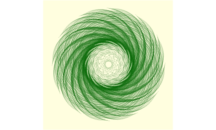
I am experimenting with generative art – essentially creating computer generated art. Here is my first creation – I am calling it StarCircle. I love how it has a 3-D aspect to it – almost spherical.
This is created in R using the ggplot package. Code for creating this is simple enough. Caution – it does take a while to run and render even in my decently powerful home desktop.
suppressMessages(library(tidyverse))
seq(-10, 10, by = 0.01) %>%
expand.grid(x=., y=.) %>%
ggplot(aes(x=(x+9.5*sin(y)), y=(y+9.5*cos(x)))) +
geom_point(alpha=.01,
shape=20, #Shape 20 is essentially a filled circle
color="blue",
size=0)+theme_void()+
coord_polar()
I cannot claim any credits for originality here though. I am following the lead of Antonio Sánchez Chinchón.
The process for creating StarCircle was quite iterative – a lot of hit-and-miss, trial-and-error. The output is very sensitive to even small changes in code parameters. For example, let us try changing the ggplot command to the following:
seq(-10, 10, by = 0.05) %>%
expand.grid(x=., y=.) %>%
ggplot(aes(x=(x+3.1*sin(y)), y=(y+19.1*cos(x)))) +
geom_point(alpha=.01,
color="darkgreen",
size=0)+theme_void()+
coord_polar()
The code above leads to this beautiful delicate Green Butterfly: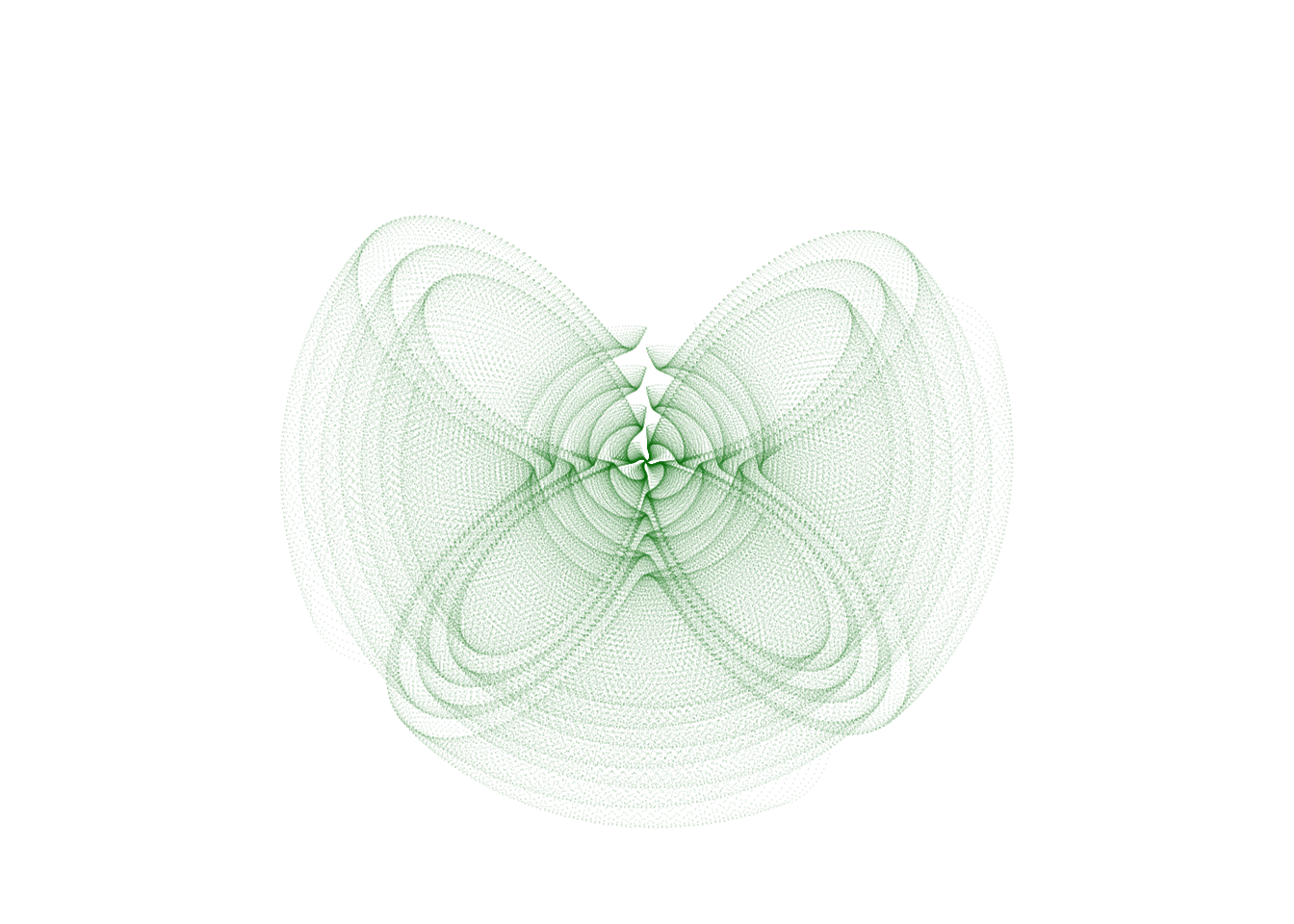 I am teaching two courses in Data Visualization in Fall. This is part of my ongoing efforts to include more creative elements in those courses. Especially for the course TO404: Big Data Manipulation and Visualization as the course is based on R and this content will fit right in.
Here is a red version of StarCircle: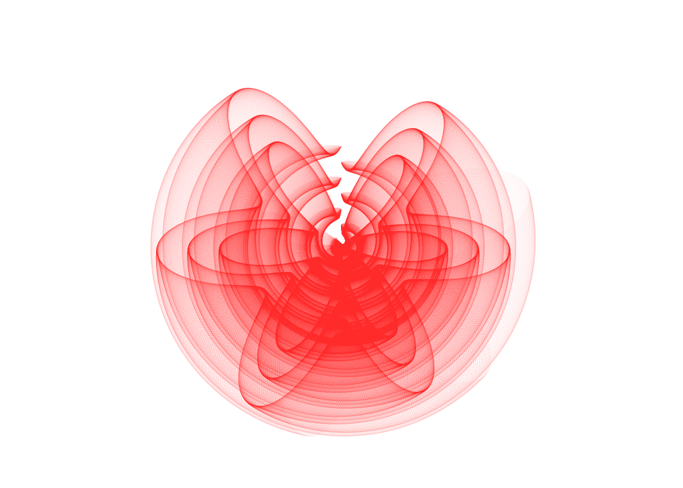
More generative art below the fold.
Update: Experiments Continuing
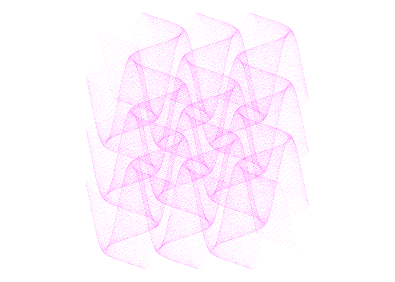
Mountains Forming
seq(-10, 10, by = 0.05) %>%
expand.grid(x=., y=.) %>%
ggplot(aes(x=(x+3.1*sin(y)), y=(y+5.1*sin(x)))) +
geom_point(alpha=.05,
           shape=20,
color="magenta",
size=0)+theme_void()+
coord_equal()
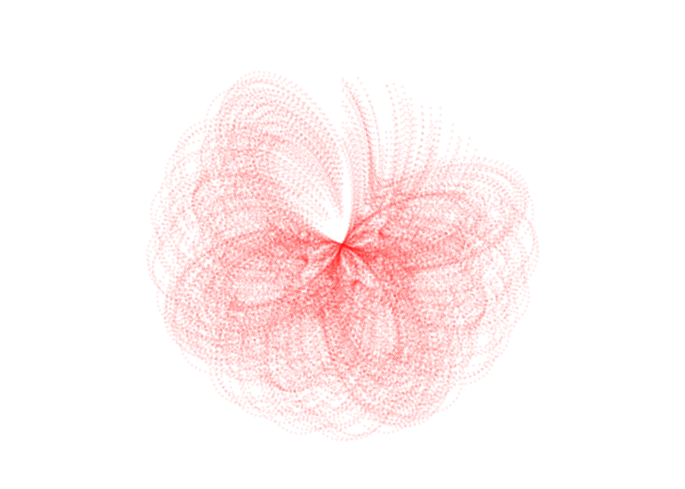
FlightPath
seq(-10, 10, by = 0.1) %>%
expand.grid(x=., y=.) %>%
ggplot(aes(x=(x+3.1*sin(y*y)), y=(y+15.1*sin(x)))) +
geom_point(alpha=.05,
           shape=20,
color="red",
size=1)+theme_void()+
coord_polar()
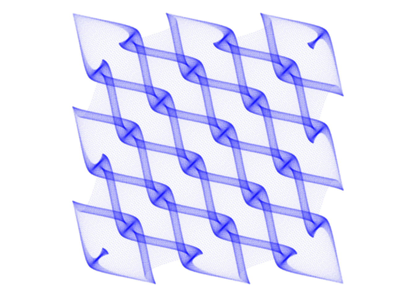
NotKnots
seq(-8, 8, by = 0.05) %>%
expand.grid(x=., y=.) %>%
ggplot(aes(x=(x+sin(y+2*x)), y=(y+sin(x+2*y)))) +
geom_point(alpha=.05,
           shape=20,
color="blue",
size=1)+theme_void()+
coord_fixed()
Tornado
seq(-12, 12, by = 0.1) %>%
expand.grid(x=., y=.) %>%
ggplot(aes(x=(cos(y+x)+1.3*y), y=(sin(x+y)+2.3*x))) +
geom_point(alpha=.05,
           shape=20,
color="red",
size=1)+theme_void()+
coord_polar()
Dispersion
seq(-12, 12, by = 0.1) %>%
expand.grid(x=., y=.) %>%
ggplot(aes(x=(sin(y+x)+y*y), y=(sin(x+y)+2.3*x))) +
geom_point(alpha=.05,
color="orangered",
size=1)+theme_void()+
coord_polar()

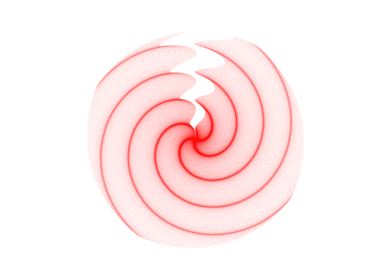
Sudarshan
This one is different as it is made with Purr. Have followed code example provided here: https://fronkonstin.com/2019/03/27/drrrawing-with-purrr/